Goal

This is part 2 of 6 in our tutorial on Arabic RAG. I’ll be using this blog as a guide, but to actually run this tutorial, its best that you run this notebook as described in part 1.

In this blog you will learn:

• How to choose an Embedding Model
• Why you need to think about token analysis for Arabic RAG
• How to analyze a tokenizer to estimate words per token
• How to visualize this to justify your decisions

Why Analyze Tokenization?

Arabic is a morphologically rich language! One of the consequences of this is that when we tokenize the words into sub-word parts, we might get lots of tokens or closer to the number of words depending on how it was written. This of course also depends on the tokenizer. If you dont know what a tokenizer is, feel free to read about it in the 🤗 NLP Course.

Embedding Model Choice

Before we analyze the tokenizer, we first need to choose an embedding model as the tokenizer is determined by the embedding model. There are a number of objectives when choosing an embedding model.

• Context window (how much text we can fit into a single embedding)
  • For some texts we might prefer the longer context window models like text-embedding-ada-002 or jinaai/jina-embeddings-v2-base-en
  • Careful as often times fitting a large amount of text into a small vector is non-trivial
• Model Size
  • Smaller models run faster, larger ones run slower
• Embedding Dimensions
  • Lower dimensions ru faster, higher ones run slower
• Model Performance
  • Usually we want the best performing model
  • Check out the MTEB Leaderboard to find the best model
• Multi-linguality
  • Obviously you may need a multi-lingual model

We obviously will prioritize multi-lingual models. To choose one lets look at the STS task tab. That’s semantic textual similarty, it tells us how good the model is at comparing similar and dissimilar text. We don’t want English only models so lets go to the Other tab. Lets sort by STS17 (ar-ar) as that is our task of choice. Now we can start to compare on other objectives we can see that sentence-transformers/paraphrase-multilingual-MiniLM-L12-v2. is the top performing model. Its also quite small and efficient! That was lucky. It’s an old model, so I do hope it gets passed soon on the leaderboard 🤞🏾

Tokenizer Analysis

Our main goal here is to answer, what is a smart MAX_WORD_LENGTH for a chunk? If we pick too few then we aren’t fully leveraging our embedding model. If we choose too many, we will be throwing away information. We want to see how many words can fit inside the context window of our model.

Why don’t we know this already? It’s because our model operates on tokens. Tokenizing all ~2.2M articles would be quite a chore, so instead we use words instead to make decisions. But how many tokens are in a word? That’s what we need to analyze. It will vary but we need to pick a smart choice.

Imports

import json
from pathlib import Path
import pickle
from tqdm.auto import tqdm

from haystack.nodes.preprocessor import PreProcessor

proj_dir = Path.cwd().parent
print(proj_dir)

Config

files_in = list((proj_dir / 'data/consolidated').glob('*.ndjson'))
folder_out = proj_dir / 'data/processed'

Load data

with open(files_in[0], 'r') as f:
    articles = [json.loads(line) for line in f]

from pprint import pprint
article = articles[0].copy()
# Truncate content so it displays well
article['content'] = article['content'][:50] + '...'
pprint(article)

{'content': 'الماء مادةٌ شفافةٌ عديمة اللون والرائحة، وهو المكو...',
 'meta': {'id': '7',
          'revid': '2080427',
          'title': 'ماء',
          'url': 'https://ar.wikipedia.org/wiki?curid=7'}}

Analysis

To figure out the tradeoffs, I’m breaking taking our first 100k articles and taking SAMPLES_PER_WORD_COUNT samples per word count to understand the token distribution. Again Arabic is a morphologically rich language, so we can expect some variance here.

Here is the idea:

1. From the first 100k articles
2. Take a random article, take a random contiguous sample of words
3. repeat step 2 SAMPLES_PER_WORD_COUNT times
4. calculate the number of tokens
5. repeat for word_lengths in range(150, 275)

Then we will have some distributions per word_length that will tell us the probability of going over our limit of 512 tokens as determined by the model.

%%time
import random
from transformers import AutoTokenizer

SAMPLES_PER_WORD_COUNT = 2000

# Each article is a dictionary with a 'content' key
# Sample: articles = [{"content": "Article 1 text..."}, {"content": "Article 2 text..."}]

tokenizer = AutoTokenizer.from_pretrained("sentence-transformers/paraphrase-multilingual-MiniLM-L12-v2")

def get_random_sample(article, length):
    words = article.split()
    if len(words) <= length:
        return None  # Skip short articles
    start_index = random.randint(0, len(words) - length)
    return ' '.join(words[start_index:start_index+length])

token_counts = {}

for word_length in range(150, 275):  # from 150 to 450 words inclusive
    token_counts[word_length] = []
    for _ in range(SAMPLES_PER_WORD_COUNT):
        article = random.choice(articles)['content']
        sample = get_random_sample(article, word_length)
        if not sample:
            continue  # Skip the iteration if the article is too short
        tokens = tokenizer.tokenize(sample)
        token_counts[word_length].append(len(tokens))

# print(token_counts)

CPU times: user 1min 12s, sys: 62.8 ms, total: 1min 12s
Wall time: 1min 12s

import plotly.io as pio
pio.renderers.default = 'jupyterlab'

import numpy as np
import plotly.graph_objects as go

# Assuming token_counts is already defined as per previous sections
word_counts = list(token_counts.keys())
all_token_counts = [token_counts[count] for count in word_counts]

# Calculate z-scores for 512 for each word count's token counts
z_scores = {}
for count, counts in zip(word_counts, all_token_counts):
    mean = np.mean(counts)
    std = np.std(counts)
    z_scores[count] = (512 - mean) / std

# Violin plot
fig = go.Figure()

for count, counts in zip(word_counts, all_token_counts):
    z_score_512 = z_scores[count]
    hover_text = f"Word Count: {count}<br>Mean: {np.mean(counts):.2f}<br>Std Dev: {np.std(counts):.2f}<br>Z-score for 512: {z_score_512:.2f}"
    
    fig.add_trace(go.Violin(
        y=counts,
        name=str(count),
        box_visible=True,
        meanline_visible=True,
        hoverinfo="text",
        text=hover_text
    ))

# Add a horizontal line at y=512 using relative positioning
fig.add_shape(
    type="line",
    x0=0,
    x1=1,
    xref="paper",
    y0=512,
    y1=512,
    line=dict(color="Red", width=2)
)

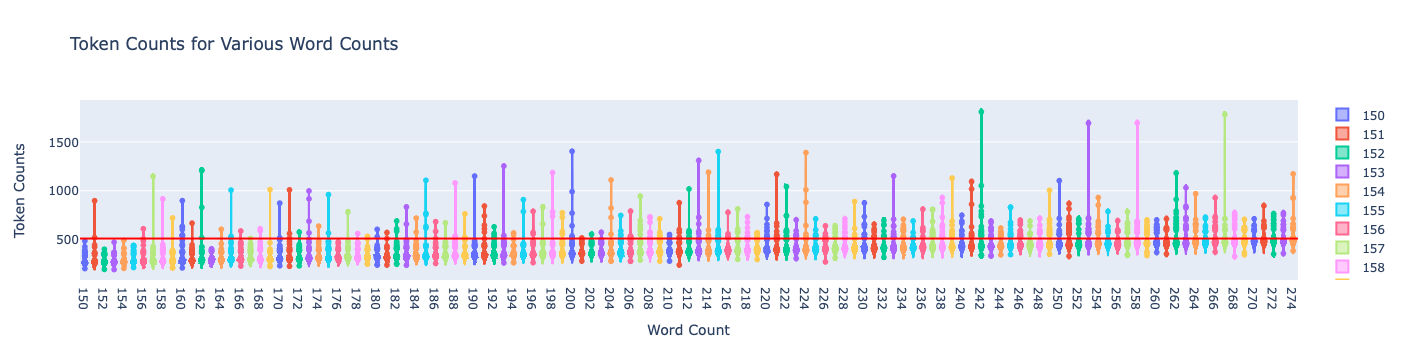
fig.update_layout(
    title="Token Counts for Various Word Counts",
    xaxis_title="Word Count",
    yaxis_title="Token Counts"
)
fig.show()

Violin plots are an aesthetic way to compare distributions for each word_length. If you run this in the notebook you can hover to see the z-scores and zoom in! Since we just have the images in this blog I put a red line for visualization purposes.

# Assuming token_counts is already defined as per previous sections
word_counts = list(token_counts.keys())
all_token_counts = [token_counts[count] for count in word_counts]

# Calculate z-scores for 512 for each word count's token counts
z_scores_list = []
for count, counts in zip(word_counts, all_token_counts):
    mean = np.mean(counts)
    std = np.std(counts)
    z_score_512 = (512 - mean) / std
    z_scores_list.append(z_score_512)

# Bar chart
fig = go.Figure(go.Bar(
    x=word_counts,
    y=z_scores_list,
    text=np.round(z_scores_list, 2),
    textposition='auto',
    marker_color='royalblue'
))

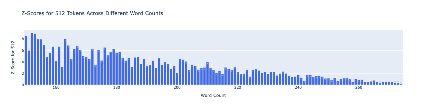
fig.update_layout(
    title="Z-Scores for 512 Tokens Across Different Word Counts",
    xaxis_title="Word Count",
    yaxis_title="Z-Score for 512"
)
fig.show()

In this chart I plot the z-score for the value of 512 for each distribution. We should expect some variance (like non-monotonicity) here since we are taking different samples for each word count. There is no right answer, but I’m feeling optimistic around 225, though some might call me a square ;)

Next steps

In the next blog post we will talk about pre-processing. This is the most underrated part of RAG IMO. That said for Wikipedia its not as challenging as say pdf types and other challenging formats. Let me know what you think in the comments!